basic formula and delta

There are plenty of articles about how to drive uniswap v3 lp values. In this post, we add some modifications to simplify future calculations.

1. your init investment value is V0=$1
2. token0 is usdc, token 1 is eth, price is usdc based eth price
3. init price is 1. All prices are generalized by init price. namely, the lower boundary is L=PL/S0.

Obviously, its delta is:

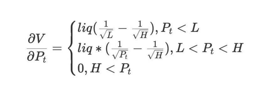
We can get a negative delta by debt. Debt's delta is always -1 per share. If you have one eth debt, you can exchange it into usdc, and profit from the eth price going down.

Asset flow

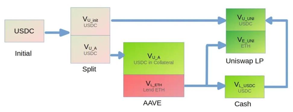
The idea is quite simple with the following steps:

1. deposit some USDC into aave and lend some eth
2. exchange some lent eth into USDC
3. the left eth and usdc go into uniswap v3 pool

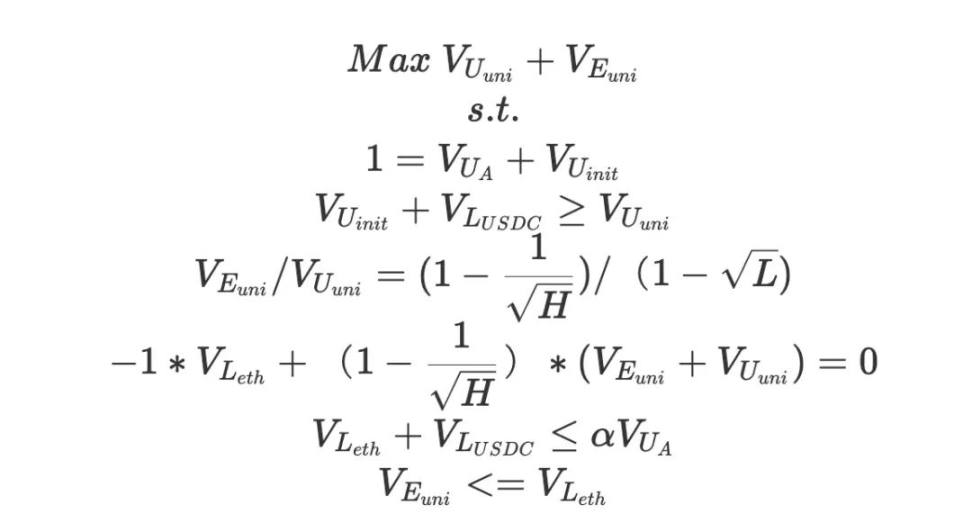
constraints an object

For an optimization problem, it includes constraints and object function.

constraint #1

init capital is $1. So we have:

constraint #2

Aave has a clearing line or risk parameter called by aave. It says that if you deposit $100 value usdc, you can only borrow α value eth.So we have

Beware that we have an eth debt as

,and exchange

constrain #3

delta neutral.

and We only care the case the price still in range. We simplify above equation as:

constrain #4

uniswap v3's rule about P,L and spot price,which is set as 1 at init:

Object function , we should max the liquidity to earn more fees. It comes out as a standard optimization problem as following:

def optimize_delta_netural(ph, pl, alpha,delta = 0.0):
    uni_amount_con = (1 - 1 / ph ** 0.5) / (1 - pl ** 0.5)

    liq = 1/(2 - 1 / sqrt(ph) - sqrt(pl))
    # solution x
    # V_U_A: value go into AAVE 0
    # V_U_init: init usdc , not go into AAVE 1
    # V_U_uni: usdc in uniswap 2
    # V_E_uni: eth in uniswap 3
    # V_E_lend: eth lend from aave 4
    # V_U_lend: some eth lend from aave exchange to usdc 5

    # V_U_A = x[0]
    # V_U_init = x[1]
    # V_U_uni = x[2]
    # V_E_uni = x[3]
    # V_E_lend = x[4]
    # V_U_lend = x[5]

    # add constrains
    cons = ({"type": "eq", "fun": lambda x: x[0] + x[1] - 1},  # V_U_A + V_U_init = 1
            {"type": "eq", "fun": lambda x: x[2] * uni_amount_con - x[3]},  # uniswap providing constrain
            {"type": "eq", "fun": lambda x: (1 - 1 / ph ** 0.5) * (x[2] + x[3]) * liq - (x[5] + x[3])-delta},  # delta netural
            # ineq
            {"type": "ineq", "fun": lambda x: x[1] + x[5] - x[2]},  # amount relation for usdc
            {"type": "ineq", "fun": lambda x: x[4] - x[3]},  # amount relation for eth
            {"type": "ineq", "fun": lambda x: alpha * x[0] - x[5] - x[4]},  # relation for aave
            # all x >= 0
            {"type": "ineq", "fun": lambda x: x[0]},
            {"type": "ineq", "fun": lambda x: x[1]},
            {"type": "ineq", "fun": lambda x: x[2]},
            {"type": "ineq", "fun": lambda x: x[3]},
            {"type": "ineq", "fun": lambda x: x[4]},
            {"type": "ineq", "fun": lambda x: x[5]},
            )

    init_x = np.array((0, 0, 0, 0, 0, 0))
    # # Method Nelder-Mead cannot handle constraints.
    res = minimize(lambda x: -(x[2] + x[3]), init_x, method='SLSQP', constraints=cons)

Optimization  demo

We choose making range as (0.9,1.1), and aave risk parameter as 0.7. the solution is

We can see that about 83% init investment goes into liquidity providing.

gamma and theta

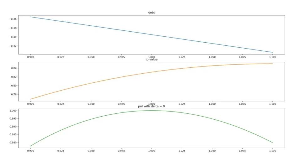
Figure 1 shows the variation of the borrowing balance with price changes, Figure 2 shows the variation of the Uniswap LP's value with price changes, and Figure 3 shows the total value of both. From the figures, it can be observed that when the price fluctuates by 10%, the total net value changes by approximately 2%.After delta hedging, the v3 LP becomes a pure short Gamma strategy.

So, can the fee income cover the 2% loss caused by a 10% price drop? Before conducting empirical backtesting, let's discuss the gamma-theta trade-off.

Since we have implemented delta hedging, and assuming constant volatility, we can derive:

With this formula, we can determine how much the price of ETH changes within a day causes us a potential loss.

Backtesting

In the latest release, our open-source software Demeter^[1] has integrated lending protocols. We can backtest our theoretically delta-neutral strategy to evaluate its performance.

Demeter feature：

• Backtrader style: Backtrader style interface makes it easier for users to get started.
• Broker/market: Demeter draws on the concepts of brokers and markets from real markets. The broker holds the asset and provides various markets to invest in. Demeter supports a variety of markets, including Uniswap and Aave, and more markets are coming. Users can test strategies for investing in multiple markets.
• Data feeding: Backtesting requires real market data. Thanks to the transparency of the blockchain, this data can be fetched from event logs of transactions. We provide demeter-fetch to do this work. It can download event logs from RPC or Google BigQuery and decode them into market data.
• Uniswap market: As a popular automated market maker, Uniswap is famous for its complexity. To raise the fund utilization rate, Uniswap adds ticks range to the position, which makes it difficult to estimate the return on investment. Demeter provides comprehensive calculation and evaluation tools to help users test the returns of various positions.
• Aave market: Aave is a popular liquidity protocol that allows users to deposit and borrow assets. By supplying assets to Aave, users can earn interest, and borrowing allows users to earn extra profit or hedge price changes. Demeter supports supply/repay/borrow/repay/liquidation transactions on Aave.
• Accuracy: In the design of Demeter, accuracy is an important consideration. In order to provide higher accuracy, the core calculations of Uniswap and Aave do not follow theoretical formulas but draw on the code of the contract. This allows Demeter to have higher calculation accuracy.
• Indicators: Besides simulating the DeFi market, Demeter also provides various indicators. These indicators will help users decide how and when to make transactions and evaluate their strategies.
• Rich interface in strategy: In the strategy, Demeter provides a lot of interfaces, which help users write strategies freely. With triggers, users can make transactions at a specified time or price. With the on_bar and after_bar functions, users can check and calculate on each iteration. Initialize and finalize functions are also provided.

Code

class DeltaHedgingStrategy(Strategy):
    def __init__(self):
        super().__init__()
        # calculate numbers about delta hedge
        optimize_res = optimize_delta_netural(float(H), float(L), float(AAVE_POLYGON_USDC_ALPHA))
        V_U_A, V_U_init, V_E_lend, V_E_uni, V_U_lend = optimize_res[1]

        self.usdc_aave_supply = Decimal(V_U_A)
        self.usdc_uni_init = Decimal(V_U_init)
        self.eth_uni_lp = Decimal(V_E_uni)
        self.eth_aave_borrow = Decimal(V_E_lend)
        self.usdc_aave_borrow = Decimal(V_U_lend)

        self.last_collect_fee0 = 0
        self.last_collect_fee1 = 0
        self.change_history = pd.Series()

    def initialize(self):
        new_trigger = AtTimeTrigger(time=datetime.combine(start_date, datetime.min.time()), do=self.change_position)
        self.triggers.append(new_trigger)

    def reset_funds(self):
        # withdraw all positions, Omitted for simplicity
        pass

    def change_position(self, row_data: RowData):
        self.reset_funds()

        pos_h = H * row_data.prices[eth.name]
        pos_l = L * row_data.prices[eth.name]

        total_cash = self.get_cash_net_value(row_data.prices)

        # invest positions
        self.last_aave_supply_value = total_cash * self.usdc_aave_supply
        self.last_aave_borrow_value = self.last_aave_supply_value * AAVE_POLYGON_USDC_ALPHA

        market_aave.supply(usdc, self.last_aave_supply_value)
        market_aave.borrow(eth, self.last_aave_borrow_value / row_data.prices[eth.name])

        self.last_net_value = total_cash

        market_uni.sell(self.usdc_aave_borrow * total_cash / row_data.prices[eth.name])  # eth => usdc

        market_uni.add_liquidity(pos_l, pos_h)

        # result monitor
        self.change_history.loc[row_data.timestamp] = "changed"
        pass

    def get_cash_net_value(self, price: pd.Series):
        return Decimal(sum([asset.balance * price[asset.name] for asset in broker.assets.values()]))

    def get_current_net_value(self, price):
        # get principle
        return Omitted_for_simplicity

    def on_bar(self, row_data: RowData):
        # reset if loss 2%
        if not self.last_net_value * Decimal("0.98") < self.get_current_net_value(row_data.prices) < self.last_net_value * Decimal(
                "1.02"):  
            self.change_position(row_data)
        pass

Due to the fixed range used in the above strategy, we refer to it as a static strategy. We also tested another dynamic strategy.

This strategy utilizes a theta table. Through this theta table, the optimal range for market-making can be obtained each day. When the price exceeds the predetermined range, the optimal investment ratio will be recalculated based on the previous day's optimal market-making range.

result

During the backtesting process, we used the following rules:

• Assuming an initial capital of $1000,
• Selected the usdc-eth (0.05) pool on Polygon, chosen for its high trading volume and representativeness.
• The time range was from August 1, 2023, to October 1, 2023, during which there were periods of stability and periods of significant price fluctuations.

In the backtesting of the static strategy, we chose a loan coefficient of 0.7 and a market-making range of [0.9 ~ 1.1]. The results are shown in the graph:

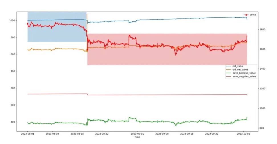
As can be seen, due to the wide selection range, there were not many position adjustments made. And during periods of significant price fluctuations, the overall net value remained relatively stable.

The final net value was 1007u, with Uniswap LP fee income of 36u. It is worth noting that on the last day of October 1st, there was a sharp increase in price, but it did not trigger a position adjustment. This resulted in a decrease in net value. If we exclude this sudden change, the net value could have reached 1016u, which corresponds to a return of 1.6% over the two months and an annualized return of 9.6%.

In the backtesting of the dynamic strategy, we also chose a loan coefficient of 0.7, and the market-making range was dynamically adjusted based on the theta table. The results are shown in the graph:

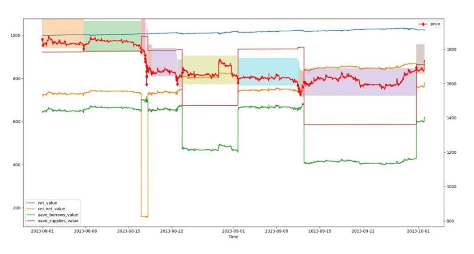
The final net value was 1024u, with Uniswap LP fee income of 65u. It generated a return of 2.4% over the two months, with an annualized return of 14.4%. Due to timely rebalancing, this strategy was minimally affected by ETH price fluctuations. For example, the price fluctuation on October 1st did not significantly impact the net value. Additionally, on August 17th, when the price sharply dropped, the strategy borrowed a significant amount of ETH and reduced investments in Uniswap, effectively hedging against the decline in ETH.

From the testing, it is evident that this strategy has a strong ability to withstand price changes. It actually generates more profit during periods of significant price fluctuations (when there is usually more swapping). If a better market-making range can be selected, the return rate can be further improved.

However, it should be noted that in this backtest, only the swap fees were considered, and the gas fees incurred during the transactions were not taken into account. Frequent operations can significantly reduce profits.

Conclusion

Using the Delta hedging strategy, it is possible to maintain the principal within a certain range of price fluctuations and earn profits from market-making on Uniswap, thereby achieving stable returns. By optimizing the market-making range, the yield can be further improved.Demeter, as an excellent backtesting tool, is simple to use and has high accuracy. It supports popular DEFI projects such as Uniswap and AAVE, and can be used to optimize investment strategies and improve investment returns.

Reference

Recommend

• • Uniswap 精翻系列

• • zkp 学习笔记

• • 研究分析专题